
Linear regression is a fundamental data analysis algorithm that predicts the value of a variable based on a linear relationship with one or more other variables. This model assumes that there is a direct linear relationship between the dependent variable and one or more independent variables, and the goal of the algorithm is to find this relationship.
The simplicity and clarity of linear regression has made it a popular tool in a variety of fields. When dealing with a single variable, linear regression is about finding the best fitting line through the data points.
Linear regression finds the best straight line (red line) that approximates the dependence between input variable X and output variable Y. This line allows predicting Y values for new X values based on the linear relationship identified (Fig. 9.3-3).

This line is represented by an equation in which inputting a value of the independent variable (X) produces a predicted value of the dependent variable (Y). This process allows Y to be effectively predicted from known values of X using a linear relationship between them. An example of finding such a statistically averaged line can be seen in the San Francisco Building Permit Data Assessment (Fig. 9.1-7), where inflation using linear regression was calculated for different types of facilities.
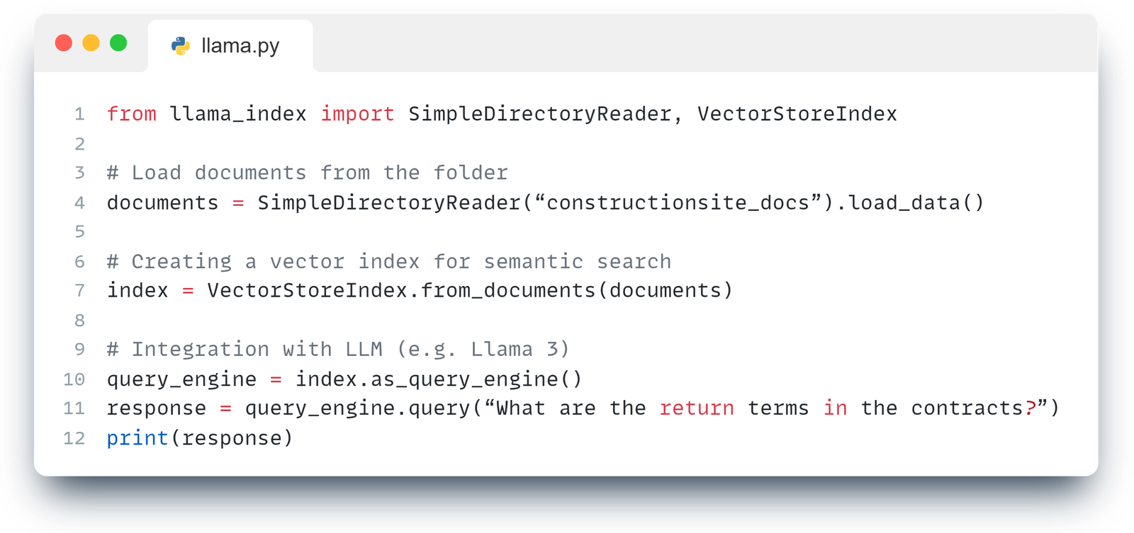
Let’s load the project data table (Fig. 9.3-2 from the previous chapter) directly into the LLM and have it build a simple machine learning model for us.
- Send a text request to LLM chat (CHATGP, LlaMa, Mistral DeepSeek, Grok, Claude, QWEN:
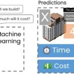
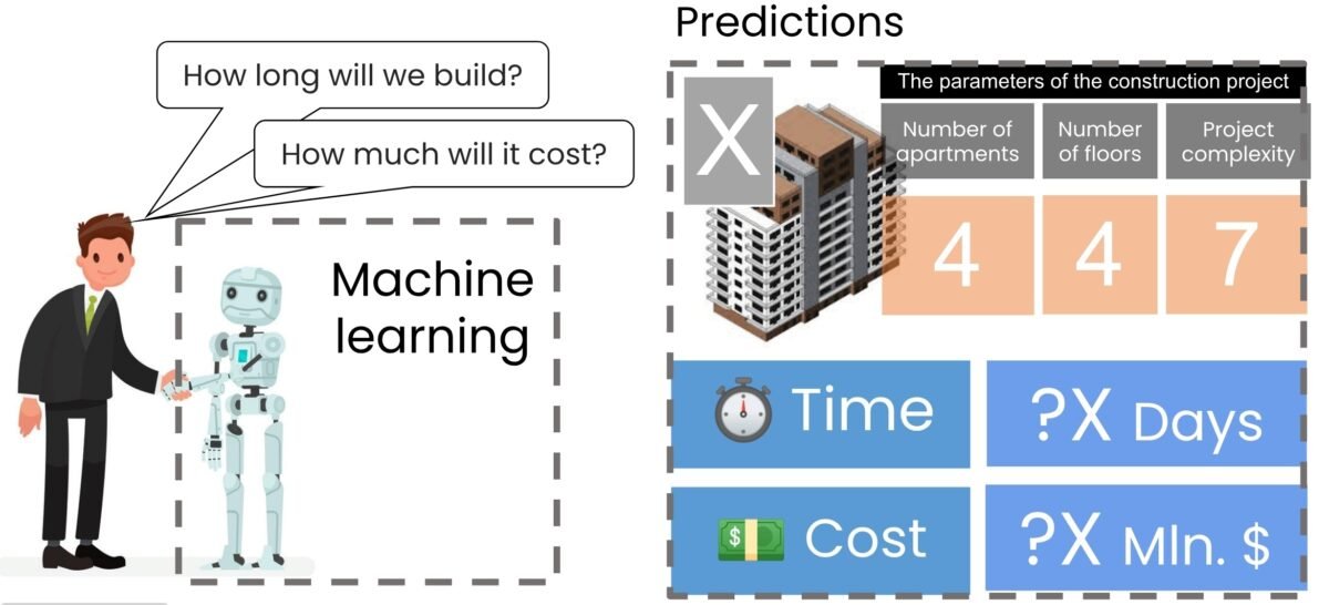
We need to show the construction of a simple machine learning model for predicting the cost and time of a new project X (Fig. 9.3-2 as attached image) ⏎
 |
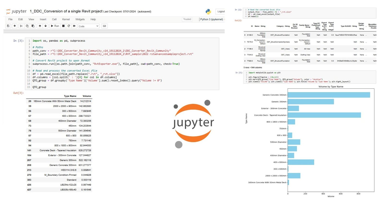
The LLM automatically recognized the table from the attached image and converted the data from a visual format to a table array (Fig. 9.3-4 – line 6). This array was used as the basis for creating features and labels from which a machine learning model was created (Fig. 9.3-4 – 17th- 22nd line), which used linear regression.
Using a basic linear regression model that was trained on an “extremely small” data set, predictions were made for a new hypothetical construction project, labeled Project X. In our problem, this project is characterized by having 40 apartments, 4 floors, and a complexity level of 7 (Fig. 9.3-2).
As predicted by a linear regression model based on a limited and small data set for the new Project X (Fig. 9.3-4 – line 24-29):
The construction duration will be approximately 238 days (238.4444444)
The total cost will be approximately $3,042,338 (3042337.777)
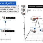
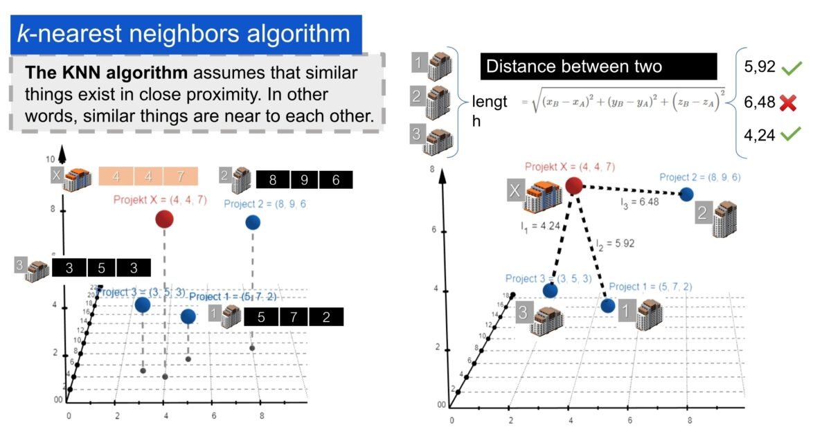
To further explore the project cost hypothesis, it is useful to experiment with different machine learning algorithms and methods. Therefore, let’s predict the same cost and time values for a new project X based on a small set of historical data using the K-Nearest Neighbours algorithm (k-NN).


